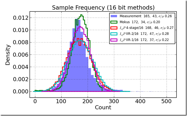
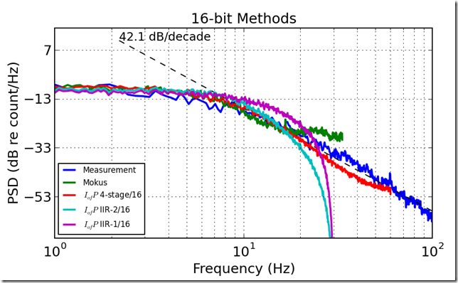
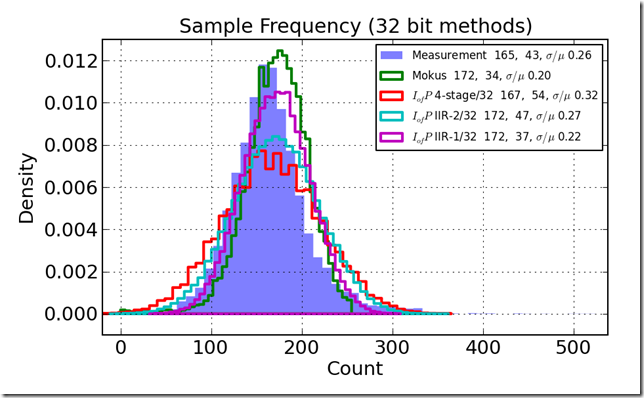
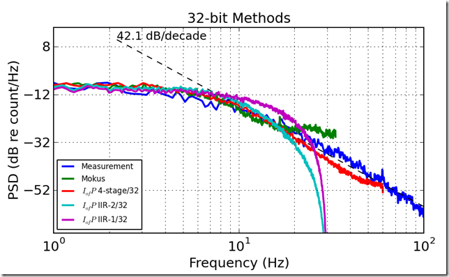
Update December 24, 2013: Mokus refined his code so that the distribution is now well-behaved (nearly normal) and the PSD no longer turns up at high frequencies). The plots and post have been updated to reflect this change. He will push code to the same link as available.
In my previous post on Candle Flame Flicker I describe the statistics of the optical intensity flicker from a candle in terms of the probability density of the brightness samples and in terms of the power spectral density of the brightness. In this article I discuss how to make an Arduino drive an LED to flicker in a way that is statistically similar to the measurements I took on a real candle.
In the measurements I observed the spectral roll-off of the candle to start between about 5 and 8 Hz, and to decline at a nominal rate of around 44 dB for each decade increase in frequency. The 2nd-order infinite impulse response filter is computationally efficient in terms of using a small amount of memory and requiring few calculations. However, the Arduino is not good at floating point arithmetic. On the Arduino, floating point is done in software, has relatively few bits of precision, and is about 4 to 40 times slower than fixed point (integer) math. It is quite difficult to find useful benchmarks. The basic process is to create white noise and then filter it to the correct spectral shape. Afterward, the signal is scaled to have the appropriate variance and offset with a constant to represent the average brightness of the “flame”.
The approach I used was to design the IIR in Python with scipy’s signal module. I specified a 2nd order lowpass Butterworth filter, specifying a cutoff frequency of 8 Hz, and a sample frequency of 60 Hz. I normalized the coefficients to work in a 16 bit integer space, following Randy Yates’ 2010 Practical Considerations in FIR Fixed Filter Implementations, mainly. From a synthesis perspective, there is some prior art. Philip Ching, a student at Cornell synthesized candle noise quite cleverly, though he neither reported nor replicated the correct statistics. A fellow with the handle Mokus did a very, very tiny implementation for a microcontroller with only 64 bytes of RAM. He helped me modify his code so I could compare his statistics, and after adjustment his spectrum and distribution match fairly well. The high-frequency of his PSD looks a little different from the other methods, but these may not be noticeable to the observer. Finally, there was Eric Evenchick’s coincidental post on hackaday. Mokus reported that Evanchick’s implementation has too slow an update rate; I noticed that Evanchick did not report on the statistics he was targeting nor what he achieved. I did not recreate his work to test.
Then, on to the tests. I really was interested in building and comparing statistics from a 16 bit implementation, a 32 bit implementation in both a Direct Form I and a Direct Form II implementation. Indeed, I had great difficulty getting the filters to perform because I kept misdesigning the integer coefficients and overflowing the registers. As I sought a solution to the 2nd-order filter approach, I also created a 4-stage digital equivalent of an RC filter. The 4-stage RC approach was always stable though it needed a higher sample rate and used much more processor power to create statistically consistent results. On the other hand, it has a more accurate spectrum. A comparison of three different 16-bit methods to Mokus’ and to the actual measurements is shown in the figure below. The legend shows the mean, standard deviation, and their ratio to the right of the label. The All my filters did a credible job of reconstructing the histogram.
The power spectral density (PSD) of the different methods tells a different story. The Direct Form II 16 bit filter is the most visually appealing of the methods I tried. It rolls off more like the physical data than the other methods, except compared to the 4-stage RC filter. The Direct Form II filter is more computationally efficient.
The results for the 32-bit versions show greater variance than the 16-bit versions, but the quality is not markedly better.
I wrote a proof code for the Arduino UNO both to see it flicker and to test the processor speed—separate parts of the code. The results are that compiling with 1.0.3 resulted in a 4,722 byte program that calculated 10,000 new values in 6,292 ms, or 629 microseconds per value. In theory this could produce a sample rate of nearly 1.6 KHz. Or another way of thinking about this is that the final code uses about 629 us/17 ms or about 4% of the processor capability of the Arduino UNO. That leaves a lot of resources available to do other Arduino work or maybe means it can fit in a cheaper processor.
I have released two pieces of code under the GNU Public License 3, you can get the Python I used for filter design and the Arduino test code at the links. If you want the data, please contact me through the comments and I am willing to provide it.


