
I have been calling my 3D response function a “surface”—which is linguistically feckless at best. Of course, I have some company, the immortal Box, Hunter, and Hunter call the experiment design a response surface method. So note carefully, the response function is not a surface, it completely fills a volume.
Naturally, this is hard to visualize. The contour plots are slices through the response space, but I really have a hard time inferring what my coffee quality function is telling me. Better visualization to the rescue.
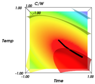
First, put the contour plots together into slices, using just the shaded parts and not the lines. Note that these cuts run through the center of the design point, and not the stationary point.
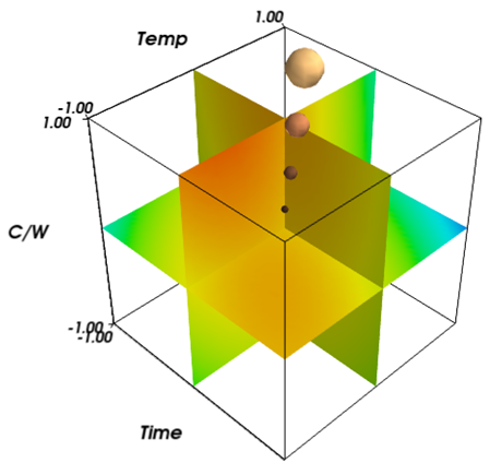
This is still quite difficult to interpret. The blue and green corners of the areas are clearly to be avoided, while the red-tinted areas near the top are to be embraced. Red, in all these plots, is a higher value of q than blue. The weird little balls are the points on the steepest ascent experiment path. Their radius corresponds to their predicted q values. Tufte, of course, would have a fit; clearly the volume should be proportional to the indicated variable.
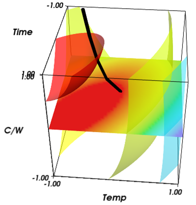
Those planar cuts are nice to look at, but we can do even better. Add “isosurfaces”—these are surfaces that lie on constant values of q. In two dimensions a topo map shows lines of constant elevation. For 3D data, the lines become surfaces. In the following figure I’ve kept the horizontal cut, and added isosurfaces. The big black line shows the steepest ascent.
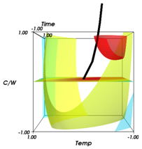
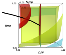
This is getting useful. To make a good cup of coffee, you want to be somewhere in the red cup on the upper-left-front corner. The zone is not enormous. To more clearly visualize this, here is the same concept from a few different angles.
So, here we are, and I still don’t have a good idea what the response function looks like outside the design space. Clearly there is a region in the middle which is relatively high quality, and it appears that higher C/W ratios are favored.
Finally, to get a solid sense of the response function I thought it would be helpful to zoom out. The next graph shows the response function in extrapolated over a much wider range.
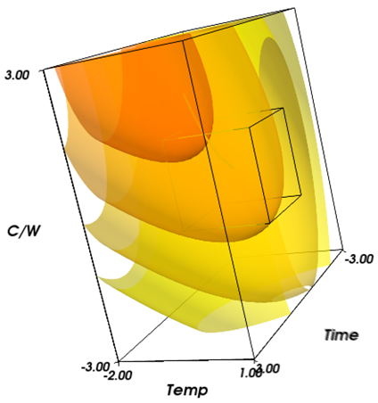
The little box in the middle is the design space. In this case there are four isosurfaces drawn, for q=1,2,3,4. With this visualization you can clearly see the shapes represented by the response function. I’m sure that the function is a poor representation of truth in the regions far from the design space. Nevertheless, this diagram is more helpful to me than any other, as I can see there is clearly a cup-shaped region in which my coffee should be really awesome. The region is surprisingly narrow over C/W ratio, time, and temperature. A poor-man’s sensitivity analysis.
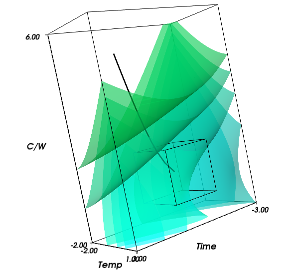
All the previous analysis has been on the response surfaces for the RSO data set only, that is, I left out the original data from the screening experiment. If I include the alternate data the fit remains qualitatively similar in that there is a tasty region in the upper left hand part of the original design space. However, the rest seems very different. There is now a saddle point, and more of the design space is better than before. Now, too, the steepest ascent path points toward increasing C/W ratio and decreasing temperature. Unlike the previous fit, though, there is substantial decrease in time inferred. Furthermore, this surface admits quality values in excess of 5. The upper isosurface is q = 5.
Resources
On the off chance you’re wondering how I made these really cool plots…
Analysis of the experiment and fitting of the response model to the data was accomplished in the wonderful language R. I couldn’t find any way to do cut-planes in R, and in any case am not terribly good with it. So I used Python(x,y) with the Enthought Tool Suite, in particular the mlab and Mayavi interfaces. Many, many thanks to the good people of the Pythonic world, and especially Enthought, for the quality product they have created. Who needs Matlab anyway?
My source code is available upon request.